Inelastic neutron-scattering from RE ions in a crystal field including damping effects due to the exchange interaction with conduction elecrons

This is an extension of the theory published by Klaus W. Becker, Peter Fulde and Joachim Keller in Z. Physik B 28,9-18, 1977 "Line width of crystal-field excitations in metallic rare-earth systems" and an introduction to the computer program for the calculation of the neutron scattering cross section. The computer program is written by J. Keller, University of Regensburg.

Here we present a brief outline of the theoretical concepts to calculate the dynamical susceptibility of the Re ions and the scattering cross section.

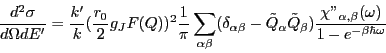
The neutron-scattering cross section is related to the dynamic susceptibility of the RE ions

$$\chi_{\alpha\beta}(t)={i\over \hbar} \Theta(t)\langle [J^\dagger_\alpha(t), J_\beta(0)]\rangle$$

whose Fourier-Laplace transform

$$\chi_{\alpha,\beta}(z)=\int_{-\infty}^{+\infty} dt e^{izt}\chi_{\alpha\beta}(t), \quad z=\omega +i\delta$$

determines the inelastic neutron scattering crossection (Stephen W. Lovesey; "Theory of neutron scattering from condensed matter" Vol 2, equ. 11,144).

$${d^2\sigma \over d\Omega d E'}= {k' \over k}({r_0\over 2}g_J... ...hi{''}_{\alpha,\beta}(\omega)\over 1-e^{-\beta \hbar \omega}}$$

Here $k$ and $k'$ denote the wave number of the neutron before and after the scattering. $\vec Q = \vec k - \vec k'$ is the scattering wave vector, $\tilde Q = \vec Q/\vert\vec Q\vert$. $r_0= -0.54 \cdot 10^{-12}$ cm is the basic scattering length, $g_J$ is the Landé factor, $F(Q)$ the atomic form factor of the rare earth ion.

Formal evaluation of the dynamic and static susceptiblity.

The dynamic spin-susceptibilities are correlation functions of the form

$$\chi_{i,k}(t)=i \Theta(t) \langle [A_i^\dagger(t),A_k(0)]\rangle$$

where $A(t)$ is a Heisenberg operator

$$A(t)= \exp(iHt)A\exp(-iHt)$$

Introducing a Liouville operator (acting on operators of dynamical variables) by ${\cal L}A = [H,A]$ the Heisenberg operator can also be written formally as

$$A(t)= \exp(i{\cal L}t) A$$

With help of this definition the dynamical susceptibility $\chi_{i,k}$ of two variables $A_i, A_k$ can be written as

$$\chi_{i,k}(t)=i \Theta(t) \langle [A_i^\dagger(t),A_k(0)]\rangle$$

and their Laplace transform

$$\chi_{i,k}(z)=i\int_0^\infty dt e^{izt} \langle [A_i^\dagger(t),A_k(0)]\rangle$$

With help of the Liouvillian these quantities can be written as

$$\chi_{i,k}(t)=i \Theta(t) \langle [A_i^\dagger,A_k\exp^{-i{\cal L}t}\rangle$$

and their Laplace transform

$$\chi_{i,k}(z)= -\langle [A_i^\dagger,{1\over {z-\cal L}}A_k(0)]\rangle$$

The static isothermal susceptibilities can also formally be calculated with help of the Liouvillian.

$$\chi_{i,k}(0) = \int_0^\beta d \lambda \langle e^{\lambda H}... ... \lambda \langle (e^{\lambda {\cal L}} A_i^\dagger) A_k\rangle$$

The static susceptibilities are used to define a scalar product between the dynamical variables:

$$(A_i \vert A_k) = {1\over \beta }\int_0^\beta d\lambda \lang... ...da{\cal L}}A_i^\dagger)A_k\rangle ={1\over \beta} \chi_{ik}(0)$$

It fulfills the axioms of a scalar product and furthermore it has the important property

$$({\cal L}A_i\vert A_k)=(A_i\vert {\cal L}A_k)={1\over \beta}\langle [A_i^\dagger,A_k]\rangle$$

With help of this relation the dynamical susceptibility can be expressed as

$$\chi_{i,k}(z)= -\beta (A_i\vert {{\cal L}\over {z-\cal L}} A_k)$$

and finally as

$$\chi_{ik}(z)=\chi_{ik}(0)-z\beta (A_i\vert {1\over {z-\cal L}}A_k)$$

The second term is the so-called relaxation function

$$\Phi_{ik}(z)=(A_i \vert {1 \over {z-\cal L}}A_k)$$

The model:

We calculate the spin susceptibility of a RE ion in the presence of exchange interaction with conduction electrons. The system is described by the Hamiltonian

$$H=H_{cf}+H_{el}+H_{el,cf}$$

The first part is the cf-Hamiltonian of the spin-system:

$$H_{cf}= \sum_n E_n K_{nn}, \quad K_{nm}= \vert n\rangle \langle m\vert$$

written in terms of the crystal field eigenstates $\vert n\rangle$. The second part is the Hamiltonian of the conduction electrons

$$H_{el}=\sum_{k\alpha}\epsilon_kc^\dagger_{k\alpha}c_{k\alpha}$$

The third part is the interaction between local moments and the conduction electrons

$$H_{el,cf}= - J_{ex}\vec J \cdot \vec \sigma, \quad \vec \sig... ...alpha}c_{k+Q\beta}, \quad \vec J=\sum_{n,m}\vec J_{n,m}K_{nm}.$$

We assume, that the energies $E_n$ and the eigenstates $\vert n\rangle$ expressed by angular momentum eigenstates are known.

Definition of dynamical variables

In our case we use as dynamical variable the standard-basis operators

$$A_\mu= K_{\mu}$$

describing a transition $\mu= [nm]$ between CEF levels $m$ and $n$. In the absence of the interaction with conduction electrons

$${\cal L}A_\mu = (E_n-E_m)A_\mu$$

In order to get the spin suceptibility we have to multiply the final expressions by the spin-matrixelements:

$$\chi_{\alpha \beta}$$

The idea of the projection formalism to calculate the dynamical susceptibility of a variable $A$ is to project this variable onto a closed set of dynamical variables $A_i$ and to solve approximately the coupled equations between these variables. For this purpose a projector is defined by

$${\cal P} A= \sum_{\nu \mu}A_\nu P^{-1}_{\nu \mu}(A_\mu\vert A) \quad P_{\nu\mu}=(A_\nu\vert A_\mu)$$

where $P^{-1}_{\nu \mu}=[P^{-1}]_{\nu \mu}$ is the ${\nu\mu}$-component of the inverse matrix of $P$.

For the resolvent operator of the relaxation function

$${\cal F}(z)= {1\over {z-\cal L}}, \quad ({z-\cal L}){\cal F}(z)=1$$

one obtains the exact equation

$$({\cal P}(z-{\cal P}{\cal L}{\cal P} - {\cal P} {\cal M}(z) {\cal P}){\cal P} {\cal F}(z) {\cal P}= {\cal P}$$

with the memory function

$${\cal M}(z)={\cal PLQ}{1\over z-{\cal QLQ} }{\cal QLP}$$

where ${\cal Q}=1-{\cal P}$. In components

$$\Phi_{\nu\mu}(z)= (A_\nu\vert {1\over z-{\cal L}} A_\mu)$$

$$\sum_\lambda \Bigl(z\delta_{\nu\lambda}-\sum_\kappa\bigl[L_{... ...]P^{-1}_{\kappa\lambda}\Bigr)\Phi_{\lambda\mu}(z) =P_{\nu \mu}$$

with

$$L_{\nu\mu}=(A_\nu\vert {\cal L}A_\mu)$$

and the memory function

$$M_{\nu\mu}(z)=(A_\nu\vert{\cal M}(z)A_\mu)$$

Now we apply the formalism to the coupled spin-electron system and restrict ourselves to the lowest order contributions of the spin electron interaction. As dynamical variables we choose a decomposition of the original spin-variable:

$$J^\alpha=\sum_{n_1,n_2}J^\alpha_{n_2,n_1}K_{n_2,n_1}=\sum_\nu J^\alpha_\nu A_\nu, \quad A_\nu= K_{n_1n_2}$$

where $\nu$ denotes a transition $n_2 \gets n_1$ performed with the standard-basis operator $\vert n_2\rangle\langle n_1\vert$.

In lowest (zeroth) order in the el-cf interaction

$${\cal L}A_\nu = (E_{n_2}-E_{n_1)}A_\nu$$

and the scalar product is diagonal in lowest order in the transition operators,

$$P_{\nu\mu}=(A_\nu\vert A_\mu)\simeq\delta_{\nu \mu}P_\nu, \q... ...(A_\nu\vert A_\nu)={p(n_1)-p(n_2)\over \beta (E_{n2}-E_{n_1})}$$

where $p(n)=\exp(-\beta E_n)/Z$ is the thermal occupation number. For the frequency term we then get

$$L_{\nu\mu}=\delta_{\nu\mu}(A_\nu\vert A_\nu) (E_{n_2}-E_{n_1} ) +O(J_{ex}^2)$$

Neglecting the second-order energy corrections in the following we obtain the equation for the relaxation function

$$\Phi_{\nu\mu}(z)=\bigl[\Omega^{-1}\bigr]_{\nu\mu}(z) P_\mu, ... ...u} - M_{\nu\mu}(z)[P^{-1}]_\mu, \quad E_\nu = E_{n_2}- E_{n_1}$$

and it remains to calculate the memoryfunction containing the relaxation processes.

In lowest order in the electron-spin interaction ${\cal QL}A_\nu$ can be replaced by ${\cal L}_{el,cf}A_\nu$. Then we get for the memory function

$$M_{\nu \mu}(z)= ({\cal L}_{el,cf}A_\nu \vert{1\over z- {\cal L}_0}{\cal L}_{el,cf}A_\mu)= M_{n_2n_1,m_2m_1}(z)$$

with

$$M_{n_2n_1,m_2m_1}(z)=({\cal L}_{el,cf} K_{n_2n_1}\vert{1\over z-{\cal L}_0}{\cal L}_{el,cf} K_{m_2m_1})$$

Now

$${\cal L}_{el,cf} K_{n_2n_1} = J_{ex}\sum_t \vec \sigma(\vec J_{n_1t} K_{n_2t} - \vec J_{tn_2}K_{tn_1})$$

with

$$\vec \sigma = \sum_{k\alpha, k+Q\beta}\vec \sigma_{\alpha\beta} c^\dagger_{k\alpha}c_{k+Q\beta}$$

With help of the symmetry properties

$$( \sigma^i K_{nm}\vert {1\over z- {\cal L}_0}\sigma^j K_{n'm'})= \delta_{ij}\delta_{nn'}\delta_{mm'}G_{nm}(z)$$

with

$$G_{nm}(z)=( \sigma^i K_{nm}\vert {1\over {z-\cal L}_0}\sigma^i K_{nm})$$

we obtain M_n_2n_1,m_2m_1(z)=J_ex^2_i[& _n_2m_2_tJ^i_m_1tJ^i_tn_1G_n_2t + _n_1m_1_tJ^i_ n_2tJ^i_tm_2G_tn_1
&-J^i_m_1n_1J^i_n_2m_2G_n_2m_1 -J^i_n_2m_2J^i_m_1n_1G_m_2n_1]

In order to calculate the relaxation functions $G_{n,m}(z)$ we use the general relation between relaxation function and dynamic susceptibility

$$\chi(z)= \chi(0)-\beta z \Phi(z)$$

and calculate instead the corresponding susceptibility (using tr $\sigma^i\sigma^i)=2$): G_nm(z)&= 2_k,k+Q [K_mn c^_k+Qc_k,(z - E_n + E_m -_k+_k+Q)^-1 K_nm c^_kc_k+Q]
&= 2 _k,Q(f_k+Q(1-f_k)p_m-f_k(1-f_k+Q)p_n)( z-E_n+E_m-_k+_k+Q)^-1 We are interested in the imaginary part describing the relaxation processes:

$$Im G_{nm}(\omega+i\delta)= - {2\pi \over \beta \omega }\sum_... ..._n \Bigr) \delta(\omega -E_n+E_m-\epsilon_{k}+\epsilon_{k+Q})$$

Writing $\rho=\omega - \omega_{nm}$ and $\omega_{nm}=E_n-E_m$ we obtain

$$Im G_{nm}(\omega+i\delta)= - {2\pi N^2(0)\over \beta \omega}... ...)(1-f(\epsilon+\rho) p_m - f(\epsilon+\rho)(1-f(\epsilon))p_n)$$

For the integrals we get df()(1-f(+)=&d ((+))/ (1+())(1+((+))
=& (-_nm)((-_nm))/ (-1+((-_nm) df(+)(1-f()=&d (()/ (1+())(1+((+))
=& (-_nm)/ (-1+((-_nm)) This makes

$$Im G_{nm}=-{2\pi N^2(0)\over \beta \omega}(\omega -\omega_{n... ...\exp(-\beta \omega)\over 1-\exp[(\omega_{nm}-\omega)\beta]}p_m$$

which has to be used to calculate the imaginary part of the memory function. Writing

$$F_{nm}(\omega )= {1\over \beta \omega}(\omega -\omega_{nm}) {1-\exp(-\beta \omega)\over 1-\exp[(\omega_{nm}-\omega)\beta]}p_m$$

which also be written in symmetrized form as

$$F_{nm}(\omega )= {\sqrt{p_np_m}\over \beta}{(\omega -\omega_... ...\omega-\omega_{nm})/2) - \exp(-\beta (\omega -\omega_{nm})/2)}$$

we obtain with $g=J_{ex}N(0)$ M_n_2n_1,m_2m_1() =- i 2g^2 _i[& _n_2m_2_tJ^i_m_1tJ^i_tn_1F_n_2t + _n_1m_1_tJ^i_ n_2tJ^i_tm_2F_tn_1
&-J^i_m_1n_1J^i_n_2m_2F_n_2m_1 -J^i_n_2m_2J^i_m_1n_1F_m_2n_1] from which we get the memory function matrix in the space of dynamical variables

$$M_{\nu \mu}(\omega)= M_{n_2n_1,m_2m_1}(\omega)$$

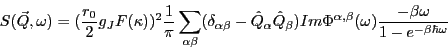
Summary: For the neutron scattering cross section we need the function $Im \chi^{\alpha\beta}(\omega+i\delta)/(1-\exp(-\beta\omega)$, where $\chi^{\alpha\beta}(z)$ is the frequency dependent part of the dynamic susceptibility $\chi^{\alpha\beta}(z)$ for spin components $J^\alpha$,$J^\beta$, which is related to the corresponding relaxation function $\Phi^{\alpha,\beta}$ by

$$\chi^{\alpha\beta}(z) = \chi^{\alpha\beta}(0) - \beta z \Phi^{\alpha\beta}(z)$$

For the full dynamical susceptibility we need the static suseptibility $\chi^{\alpha\beta}(0)$ which in lowest order in the exchange interaction is given by

$$\chi^{\alpha\beta}(0) = \sum_\nu (J^\alpha_\nu)^\dagger \beta P_\nu J^\beta_\nu$$

The above relaxation function is calculated with help of the Mori-Zwanzig projection formalism by

$$\Phi^{\alpha\beta}(z)=\sum_{\mu\nu} (J^\alpha_\nu)^*\Phi_{\nu\mu}(z)J^\beta_\mu$$

where $\nu$ denotes a transition from $n_1$ to $n_2$ between crystal field levels of the magnetic ion. The partial relaxation functions are obtained by solving the matrix equation

$$\Phi_{\nu\mu}(z)= [\Omega^{-1}]_{\nu\mu}P_\mu$$

with

$$\Omega_{\nu\mu}(z)= (z-\omega_\nu)\delta_{\nu\mu} -M_{\nu\mu}(z)/P_\mu$$

where $\omega_\nu =E_{n_2}- E_{n_1}$ is the energy difference of cf-levels.

Only terms in lowest order in the el-ion interaction are kept. We neglect frequency shifts due to the electron-ion interaction. Then the memory function is purely imaginary (with a negative sign).

Note that compared to our paper BFK, Z.Physik B28, 9-18, 1977 we have used here a different sign-convention.

For numerical reasons it is more convenient to calculate the relaxation function in the following way:

$$\Phi_{\nu\mu}(z)= P_\nu[\bar\Omega^{-1}]_{\nu\mu}P_\mu$$

with

$$\bar \Omega_{\nu\mu}(z)= P_\nu(z-\omega_\nu)\delta_{\nu\mu} - M_{\nu\mu}(z)$$

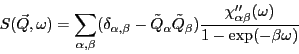
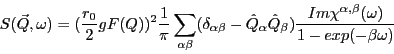
From the relaxation function we get for the dynamic scattering cross section

$${d^2\sigma \over d\Omega d E'} = {k' \over k}S(\vec Q,\omega)$$

with

$$S(\vec Q, \omega)=({r_0\over 2}g_J F(\kappa))^2{1\over \pi }... ...\beta}(\omega){-\beta \omega \over 1-e^{-\beta \hbar \omega}}$$

Here the scattering function depends only on the scattering vector $\vec Q = \vec k - \vec k'$ and the energy loss $(\hbar)\omega =E(k)-E(k')$ Note that in our formulas $\omega$ contains a factor $\hbar$ and is the energy loss. If we want to have meV as energy unit and Kelvin as temperature unit, we have to write $\beta= 11.6/T$.

For the analysis of polarised neutron scattering the different spin-components $S^{\alpha\beta}(\vec Q,\omega)$ of $S$ are needed. These are defined by

$$S(\vec Q,\omega)= \sum_{\alpha\beta}(\delta_{\alpha\beta} - \hat Q_\alpha \hat Q_\beta)S^{\alpha\beta}(\vec Q,\omega)$$

with

$$S^{\alpha\beta}(\vec Q,\omega)= Im \chi^{\alpha\beta}/(1-e^{... ...\beta}(\omega){-\beta \omega \over 1-e^{-\beta \hbar \omega}}$$

The complex dynamic susceptbility is calculated from

$$\chi^{\alpha\beta}(\omega)= \chi^{\alpha\beta}(0)-\beta \ome... ...ha_\mu)^*(P_{\mu\nu}-\omega \Phi_{\mu\nu}(\omega ))J^\beta_\nu$$

where the static susceptibilities $\beta P_{\mu\nu}$ are diagonal in our approximation.

Description of the program:

The program calculates the dynamical susceptibility and the neutron scattering cross-section of single RE ions in the presence of crystal fields and Landau damping due to the exchange interaction with conduction electrons.

It needs the following input-files (not all are needed for all tasks)

1. A file containing the information about the RE ion: Type of ion, number of CF-levels, energy eigenvalues and eigenstates. The date are extracted from the input-file by reading the information contained in lines starting with $\char93 !$ or blanks, see the attached example.

2. File with the formfactor data for RE ion

3. File with a list of ($\vec Q,\omega$)-values, for which the calculation shall be performed

4. A parameter-file containing the names of the files with the formfactor, the table with the ($\vec Q,\omega$)-values, the energy range, scattering direction etc., see the attached example.

5. The value of the coupling constant $g=j_{ex}N(0)$, the temperature, the mode of calculation, the form of the out-put, the name of the file with the CEF-data, the name of the parameter file are provided by the commandline, which is used to start the program.

The program consists of a number of modules and subroutines which are briefly described in the following:

1. Modules CommonData, MatrixElements, FormfactorPreparation

These modules contain definitions of global variables and arrays used in the program and in different subroutines. FormfactorPreparation also contains the subroutine FormfactorTransformation which transforms an input-file with formfactor data into a file with formfactor values for equidistant Q-values. and the function Formfac to calculate the formfactor at arbitrary Q-values.

2. Subroutine ReadData

Subroutine to read-in data needed to calculate the dynamical susceptibility and the neutron scattering cross-section.

It reads the commandline, containing the coupling $g=j_{ex}N(0)$, the temperature $T$ (in Kelvin), mode of calculation (see below), form of out-put, name of the file with RE data, name of the parameter-file (containing also the name of the file with the formfactor data). The information about the RE ion is transferred into a workfile cefworkfile.dat for inspection and use in the following runs. The data contained in the parameter-file are stored in the file bfkdata.dat. The latter two have to be given only in the first run. If they are left-out in the following runs, the are assumed to be unchanged.

3. Subroutine Matrixelements

a) Calculates angular momentum matrices jjx, jjy, jjz for the crystal-field eigenstates (2-dim arrays, dimension Ns x Ns). The three directional components are also stored in the 3-dimensional array jjj(3,Ns,Ns).

b) Calculates Boltzmann-factors $p(n)$. A cut-off in the exponent $\beta E(n)$ is introduced such that Boltzmann factors with large negative exponents are set equal to zero.

c) Defines a set of transitions $\nu$ between states n1 and n2, stored in two 1-dim arrays v1($\nu$), v2($\nu$). If both Boltzmann factors of the two states involved are zero, this transition is eliminated from the set of allowed transitions.

d) Calculates static suscepibilities $P(\mu)$ for the standard basis operators $K_{n,m}$ for the allowed transitions.

e) All these reults are stored in a file bfkmatrix.dat for examination, if something goes wrong.

4. MatrixInversionSubroutine

adapted from Numerical Recipes, to be used for the inversion of the complex matrix $\Omega_{\nu\mu}$. Called by 5.

5. Subroutine Relmatrix

Calculates the matrix relaxation function $\Phi_{\mu,\nu}(\omega)$ for the set of dynamical variables obtained from the standard basis operators for a given energy (freqency) $\omega$.

6. Subroutine Suscepcomponents

Calculates the different components of the dynamical susceptibility

$$\chi^{\alpha,\beta}(\omega) = \beta\sum_{\mu \nu}(J^\alpha)_... ...u\delta_{\mu\nu}-\omega \Phi_{\mu\nu}(\omega)\bigr]J^\beta_\nu$$

and

$$Im \chi^{\alpha\beta}(\omega)/(1-\exp(-\beta\omega))$$

7. Function Scatfunction(Q,$\omega$)

Calculates

$$S(\vec Q,\omega)= \sum_{\alpha\beta}\bigl(\delta_{\alpha\bet... ...lde Q^\beta\bigr) Im \chi^{\alpha\beta}/(1-\exp(-\beta\omega))$$

8. Subroutine OutputResults

Here the results for the dynamical susceptibility, the scattering function and the differential neutron scattering cross section for different scattering geometries are calculated, and the results written into files bfkm.res for different scattering-modes m=0-6, which are written into the subdirectory /results. Depending on the value of ms=1,2 the new results over-write the previews results or append.

Depending on the number m=0-6 (3. entry of the commandline) the following results are calculated.

mode=0: all nine components $\chi^{\alpha\beta}(\omega)$ of the complex dynamic susceptibility are calculated for $Npoint$ equidistant energies $\omega$ between $emin$ and $emax$.

mode=1: the diagonal components of $Im \chi^{\alpha\alpha}(\omega)/\tanh{\beta\omega/2}$ are calculated and the frequency integral is compared with the sum-rule

$$\sum_\alpha {1\over\pi}\int d\omega {Im \chi^{\alpha\alpha}\over \tanh(\beta\omega/2)} = J(J+1)$$

The sum-rule sometimes is not very well fulfilled, since within this approximation the Landau damping does not fall-off fast enough at large energies

mode=2: The scattering function

$$S(\vec Q,\omega)=\sum_{\alpha,\beta} (\delta_{\alpha, \beta}... ...eta){ \chi''_{\alpha \beta}(\omega)\over 1-\exp(-\beta\omega)}$$

is calculated for a given set of values for energy loss $\omega$ and scattering vector $\vec Q$ contained in a file specified in the parameterfile.

mode=3: The 9 different components of the scattering-function

$$(r_0g_JF(\vec Q)/2)^2{1\over \pi} S^{\alpha\beta}(\vec Q,\om... ...ga)= {Im \chi^{\alpha,\beta}(\omega)\over 1-exp(-\beta\omega)}$$

are calculated.

mode= 4-6: the neutron scattering cross section

$${d^2\sigma \over d\Omega d E'} = {k' \over k}S(\vec Q,\omega)$$

with

$$S(\vec Q, \omega)=({r_0\over 2}g F(Q))^2{1\over \pi } \sum_{... ...a) {Im \chi^{\alpha,\beta}(\omega)\over 1-exp(-\beta \omega)}$$

is calculated for different scattering geometries: In mode 4 the direction of the wave vector $\vec k$ and the energy $E=k^2/2m$ of the incident beam is fixed. The direction of the scattering wave vector $\vec Q$ is fixed, but the length of $\vec Q$ is variable. The wave vector of the scattered particles is $\vec k'=\vec k-\vec Q$, their energy is $E'=k'^2/2m$ and the energy loss is $\omega =E-E'$. In mode 5 the direction of the wave vectors $\vec k$ and $\vec k'$ of the incoming and scattered beam are fixed, while the energy $E'$ of the scattered beam is variable. In mode 6 the energy $E$ of the incident particles is variable and the energy $E'=k^2/2m$ of the scattered particles fixed.

How to run the program:

The translated program is started with a command-line like

bfk 0.1 10 0 1 prlevels.cef paramfile.par

with the following structure:

name of the program: bfk; coupling constant g; temperature T (in K); type of calculation: mode =1...6; type of output: mst=1 overwrite, mst=2 append new results; name of file with RE ion data; name of parameter file.

The last two entries can be skipped in later runs, if they are not changed.

The mode number mode = 1 ...6 refers to the subject of calculation. The output- number mst=1,2 refers to the type of output-storage.

The file with RE data should have the form produced by sol1on (see the attached example). The lines starting with numbers or blanks contain information, the lines starting with # are commentaries, the lines starting with #! also carry information.

The parameterfile contains additional parameters needed to run the program: energy range and number of energy values. Energies of incident or scattered particles, direction of incident or scattered particles.

mode=4: E energy of incident particles, k11,k12,k13 direction if incident particles (vector with arbitrary length), k21,k22,k23 direction of scattered particles.

mode=5: E energy of incident particles, k11,k12,k13 direction if incident particles (vector with arbitrary length), k21,k22,k23 direction of scattering vector $\vec Q$.

mode =6: E energy of scattered particles, k11,k12,k13 direction if incident particles (vector with arbitrary length), k21,k22,k23 direction of scattered particles.

The parameterfile also contains the namme of a file with a list of scattering vectors $\vec Q$ and energy loss ($\omega$) needed for mode 2,3

Finally it contains the name of a file with the formfactor of the ion.

J. Keller, May 2013