All the files described in the following procedure are available in the directory examples/ndcu2b_new/cf.
A simple input file is made up in the following:
It follows an example, we take the values
for NdCu![]() from literature [27]. Note that
if the crystal field parameters are not known, there are different
possibilities to obtain values, such as ab initio calculation,
point charge calculations (use module pointc) and fitting
to experimental data (see section 17).
from literature [27]. Note that
if the crystal field parameters are not known, there are different
possibilities to obtain values, such as ab initio calculation,
point charge calculations (use module pointc) and fitting
to experimental data (see section 17).
#!MODULE=so1ion
#<!--mcphas.cf-->
# comment followed by
# the ion type and the crystal field parameters [meV]
 IONTYPE=Nd3+
 GJ=0.727273
# - note you can also do any pure spin problem by entering e.g. IONTYPE=S=2.5
 B20=  0.116765
 B22  =  0.134172
 B40  =  0.0019225
 B42  =  0.0008704
 B44  =  0.0016916
 B60  =  0.0000476
 B62  =  0.0000116
 B64  =  0.0000421
 B66  =  0.0003662
# instead of the Stevens parameters Blm
# second order crystal field parameters Dx^2 Dy^2 and Dz^2 can be entered in meV
# - this coresponds to Hamiltonian H=+Dx2 Jx^2+Dy2 Jy^2+Dz2 Jz^2
Dx2=0.1
Dy2=0
Dz2=0.4
# the temperature in Kelvin
TEMP= 10
# if you want you can apply a magnetic field in Tesla
Bx=0
By=0
Bz=0
Note: you can also create an input file for so1ion with more comments for the crystal field parameters, the type of ion etc. This is done by running so1ion with the option -c, i.e.: so1ion -c, a help screen appears ...
 |
(7) |
Note: in this calculation energy and Q dependence
of the double differential scattering cross section are not considered and
integration over all energies and scattering angles has been performed.
In order to get a more realistic scattering intensity, the
form factor (giving a ![]() dependence), the
factor
dependence), the
factor ![]() and the Debye Waller factor
and the Debye Waller factor ![]() should be considered.
should be considered.
Here comes the output file so1ion.out:
#{-------------------------------------------------------------
#                  C F I E L D / S O 1 I O N    5.60           |
#                    A crystal field program                   |
#               __________________________________
#              |         Peter  Hoffmann          |
#              |    Forschungszentrum Juelich     |
#              |Institut fuer Festkoerperforschung|
#               __________________________________
#    O U T P U T         Tue Aug 30 12:44:30 2011
#--------------------------------------------------------------
#!Temperature of the sample       T=  10.00 Kelvin
#!Ion                    IONTYPE= Nd3+
#!Lande factor of the ion   gJ= 0.727273
#
# Total angular momentum J of the
#!Spin - orbit - level     J=  4.5
#!Electrons in 4f shell   Ne=  3
#--------------------------------------------------------------
# Parameter           :  Akq   in  meV   /a0**k
# (compare Hutchings Solid State Physics 16 (1964) 227, p 255 eq 5.5)
#!A20  =        -16.306372
#!A22  =        -18.737280
#
#!A40  =         -2.269445
#!A42  =         -1.027477
#!A44  =         -1.996875
#
#!A60  =         -0.083369
#!A62  =         -0.020317
#!A64  =         -0.073736
#!A66  =         -0.641377
#--------------------------------------------------------------
#--------------------------------------------------------------
# Parameter           :  Bkq   in  meV
#                        Bkq are the Stevens Parameters  - see Hutchings Solid State Physics 16 (1964) 227
#!B20  =          0.116765
#!B22  =          0.134172
#
#!B40  =          0.001922
#!B42  =          0.000870
#!B44  =          0.001692
#
#!B60  =          0.000048
#!B62  =          0.000012
#!B64  =          0.000042
#!B66  =          0.000366
#--------------------------------------------------------------
#--------------------------------------------------------------
# Parameter           :  Dkq   in  meV
#!D20 =         -36.330596
#!D22 =         -17.043002
#
#!D40 =         -52.832675
#!D42 =          -3.782031
#!D44 =          -5.556290
#
#!D60 =         -20.048458
#!D62 =          -0.476801
#!D64 =          -1.579686
#!D66 =         -10.148138
#--------------------------------------------------------------
#--------------------------------------------------------------
# Parameter           :  Lkq   in  meV
#                        Lkq are the Wybourne Parameters - see A. Kassmann J. Chem. Phys. 53 (1970) 4118
#!L20  =        -36.330596
#!L22  =        -17.043002
#
#!L40  =        -52.832675
#!L42  =         -3.782031
#!L44  =         -5.556290
#
#!L60  =        -20.048458
#!L62  =         -0.476801
#!L64  =         -1.579686
#!L66  =        -10.148138
#--------------------------------------------------------------
#--------------------------------------------------------------
# Parameter           :  Vkq   in  meV
# (NOT the same Vlm as in Hutchings p255 or Elliot and Stevens)
#!V20 =           0.116765
#!V22 =           0.067086
#
#!V40 =           0.001922
#!V42 =           0.000435
#!V44 =           0.000846
#
#!V60 =           0.000048
#!V62 =           0.000002
#!V64 =           0.000021
#!V66 =           0.000183
#--------------------------------------------------------------
#--------------------------------------------------------------
# Parameter           :  Wkq   in  meV   /a0**k
#!W20 =         -16.306372
#!W22 =          -9.368640
#
#!W40 =          -2.269445
#!W42 =          -0.513739
#!W44 =          -0.998438
#
#!W60 =          -0.083369
#!W62 =          -0.003386
#!W64 =          -0.036868
#!W66 =          -0.320689
#--------------------------------------------------------------
#--------------------------------------------------------------
#                Anisotropy parameters in meV.
#--------------------------------------------------------------
#         H= + Dx2 Jx ^ 2+ Dy2 Jy ^ 2+ Dz2 Jz ^ 2
#! Dx2 =          0.10
#! Dy2 =          0.00
#! Dz2 =          0.40
#
#--------------------------------------------------------------
#--------------------------------------------------------------
# Energy Eigenvalues are in  meV   .
#--------------------------------------------------------------
#!Nr of different energy levels   noflevels= 5
#!Energy shift   Eshift=                       -2.6744
#
# Because of the calibration freedom the smallest energy
# eigenvalue is shifted to zero. You can get the energy
# eigen-value of the applied eigen-value problem
# by shifting the energy by the added energy value above
#!*E( 1)=        0.0000        Degeneracy =   2 -fold
#!*E( 2)=        2.4850        Degeneracy =   2 -fold
#!*E( 3)=        4.5048        Degeneracy =   2 -fold
#!*E( 4)=        7.8548        Degeneracy =   2 -fold
#!*E( 5)=       19.1522        Degeneracy =   2 -fold
# Them with  *  marked Energy eigenvalues have a non-
# vanishing Matrix element of the Ground state E( 1).
#--------------------------------------------------------------
#
#--------------------------------------------------------------
# The orthonormal characteristic Eigenvectors  |i,r>  with
#
#             H |i,r>  = ( E  + E      ) |i,r>  , r=1 ... n
#                           i    shift                     i
#
#                            and
#
#                    <i,r|j,s> = D   D
#                                 ij  rs
#
#              D  = Kronecker- Delta function
#               ij
#
# the |i,r> are also orthonormal .
# We consider in this program  Crystal Field spliting
# at the lowest Spin-orbit-level (Ground state)
#
# 2S+1
#     L  of the calculated Ion. The |i,r> are in
#      J
#
# a more developed  Eigenfunction
#
# system  [ | J  M   > ]               ,where
#                 J     M = -J,...,J
#                        J
#                               ,
#              <  J  M   |  J  M  >  =  D    ,    .
#                     J         J        M  M
#                                         J  J
#--------------------------------------------------------------
#
# I 1, 1> =     0.0414               I 4.5  -4.5>
#          -    0.3955               I 4.5  -2.5>
#          +    0.7083               I 4.5  -0.5>
#          -    0.4563               I 4.5   1.5>
#          +    0.3633               I 4.5   3.5>
#
# I 1, 2> =     0.3633               I 4.5  -3.5>
#          -    0.4563               I 4.5  -1.5>
#          +    0.7083               I 4.5   0.5>
#          -    0.3955               I 4.5   2.5>
#          +    0.0414               I 4.5   4.5>
#
# I 2, 1> =    -0.0402               I 4.5  -4.5>
#          +    0.1455               I 4.5  -2.5>
#          +    0.5713               I 4.5  -0.5>
#          +    0.1221               I 4.5   1.5>
#          -    0.7975               I 4.5   3.5>
#
# I 2, 2> =     0.7975               I 4.5  -3.5>
#          -    0.1221               I 4.5  -1.5>
#          -    0.5713               I 4.5   0.5>
#          -    0.1455               I 4.5   2.5>
#          +    0.0402               I 4.5   4.5>
#
# I 3, 1> =    -0.0255               I 4.5  -3.5>
#          -    0.7164               I 4.5  -1.5>
#          -    0.0601               I 4.5   0.5>
#          +    0.6945               I 4.5   2.5>
#          -    0.0098               I 4.5   4.5>
#
# I 3, 2> =     0.0098               I 4.5  -4.5>
#          -    0.6945               I 4.5  -2.5>
#          +    0.0601               I 4.5  -0.5>
#          +    0.7164               I 4.5   1.5>
#          +    0.0255               I 4.5   3.5>
#
# I 4, 1> =     0.4804               I 4.5  -3.5>
#          +    0.5046               I 4.5  -1.5>
#          +    0.4065               I 4.5   0.5>
#          +    0.5712               I 4.5   2.5>
#          -    0.1522               I 4.5   4.5>
#
# I 4, 2> =    -0.1522               I 4.5  -4.5>
#          +    0.5712               I 4.5  -2.5>
#          +    0.4065               I 4.5  -0.5>
#          +    0.5046               I 4.5   1.5>
#          +    0.4804               I 4.5   3.5>
#
# I 5, 1> =     0.9866               I 4.5  -4.5>
#          +    0.1175               I 4.5  -2.5>
#          +    0.0557               I 4.5  -0.5>
#          +    0.0948               I 4.5   1.5>
#          +    0.0261               I 4.5   3.5>
#
# I 5, 2> =     0.0261               I 4.5  -3.5>
#          +    0.0948               I 4.5  -1.5>
#          +    0.0557               I 4.5   0.5>
#          +    0.1175               I 4.5   2.5>
#          +    0.9866               I 4.5   4.5>
#
#--------------------------------------------------------------
#
#!magnetic moment(mb/f.u.): mx= 0.000 my= 0.000 mz= 0.000
#
#--------------------------------------------------------------
#
#                  M A T R I X  E L E M E N T
#                  S I N G L E  C R Y S T A L
#
#--------------------------------------------------------------
#    Only the marix elements that are non-zero are written
#
#--------------------------------------------------------------
#                              2 |            2 |            2
#    a  <-->  b      |<a|J |b>|  |  |<a|J |b>|  |  |<a|J |b>|
#                         x      |       y      |       z
#--------------------------------+--------------+--------------
#    1  <-->  1       0.002008   |  36.711411   |   0.031042
#--------------------------------+--------------+--------------
#    2  <-->  1       1.949420   |   0.270090   |   2.638097
#--------------------------------+--------------+--------------
#    2  <-->  2       1.517583   |   2.490016   |   8.199948
#--------------------------------+--------------+--------------
#    3  <-->  1       1.415357   |   0.424874   |   2.727140
#--------------------------------+--------------+--------------
#    3  <-->  2      10.148894   |   8.149608   |   0.176745
#--------------------------------+--------------+--------------
#    3  <-->  3       9.078618   |  11.619418   |   0.380198
#--------------------------------+--------------+--------------
#    4  <-->  1       0.009374   |   1.424032   |   1.021019
#--------------------------------+--------------+--------------
#    4  <-->  2       2.500806   |   2.020701   |   5.118137
#--------------------------------+--------------+--------------
#    4  <-->  3       0.239888   |   0.004479   |   4.938522
#--------------------------------+--------------+--------------
#    4  <-->  4      26.164401   |   0.690989   |   0.070056
#--------------------------------+--------------+--------------
#    5  <-->  1       0.710568   |   0.137243   |   0.028325
#--------------------------------+--------------+--------------
#    5  <-->  2       2.282293   |   2.029398   |   0.008264
#--------------------------------+--------------+--------------
#    5  <-->  3       0.057679   |   0.000101   |   0.138477
#--------------------------------+--------------+--------------
#    5  <-->  4       3.524062   |   1.023958   |   0.749577
#--------------------------------+--------------+--------------
#    5  <-->  5       0.060712   |   0.019195   |  38.730148
#--------------------------------------------------------------
#
#
#--------------------------------------------------------------
#
#                  M A T R I X  E L E M E N T S
#                    P O L Y C R Y S T A L
#
#--------------------------------------------------------------
#
#                             ----                2
# Matrix element       :      >     |<i,r|J |k,s>|
#                             ----         T
#                              r,s
#
#
# for the transition :      E  ->  E
#                              i      k
#
#--------------------------------------------------------------
#
#                         SUm rule :
#
#             ----                2       2
#             >     |<i,r|J |k,s>|  = n  --- J(J+1)
#             ----         T           i  3
#             k,r,s
#--------------------------------------------------------------
#-----------------------------
# \ E |   |   |   |   |   |Zei|
#E \ k|E  |E  |E  |E  |E  |len|
# i \ | 1 | 2 | 3 | 4 | 5 |sum|
#----|---|---|---|---|---|---|
#| E  | 24|  3|  3|  1|   | 33|
#|  1 |.50|.24|.04|.64|.58|   |
#|----|---|---|---|---|---|---|
#| E  |  3|  8| 12|  6|  2| 33|
#|  2 |.24|.14|.32|.43|.88|   |
#|----|---|---|---|---|---|---|
#| E  |  3| 12| 14|  3|   | 33|
#|  3 |.04|.32|.05|.46|.13|   |
#|----|---|---|---|---|---|---|
#| E  |  1|  6|  3| 17|  3| 33|
#|  4 |.64|.43|.46|.95|.53|   |
#|----|---|---|---|---|---|---|
#| E  |   |  2|   |  3| 25| 33|
#|  5 |.58|.88|.13|.53|.87|   |
# ----------------------------
#
#
#
#--------------------------------------------------------------
#               Transition intensities in barn.
#
#
#
#
# =                    - E /T     -----
# |                   e   i       \                   2
# |     = const --------------     >    |<i,r|J |k,s>|
# |             ----    - E /T    /            T
# =             >    n e   i      -----
#  E -> E       ----  i            r,s
#   i    k       i
#
#                            with
#
#
#                                -----
#                      2     2   \                    2
#        |<i,r|J |k,s>|   = ---   >     |<i,r|J |k,s>|
#               T            3   /             u
#                                -----
#                             u = x,y,z
#
#
#                             und
#
#                                   1          2
#                  const  = 4*pi*( --- r   g  )
#                                   2   0   J
#
#                                      -12
#                  r      = - 0.54 * 10    cm
#                   0
#
#--------------------------------------------------------------
#
#                       1.Sum rule :
#                                                 - E /T
#                                            n   e   i
#  ----  =            2                       i
#  >     |         = --- * const * J(J+1) * ----------------
#  ----  =            3                     ----     - E /T
#   k     E -> E                            >    n  e   i
#          i    k                           ----  i
#                                            i
#--------------------------------------------------------------
#
#                       2. sum rule :
#
#
#            ----  =            2
#            >     |         = --- * const * J(J+1)
#            ----  =            3
#             k,i   E -> E
#                    i    k
#--------------------------------------------------------------
#--------------------------------------------------------------
#!Temperature of the sample               T=   10.00 Kelvin
#--------------------------------------------------------------
#!parition function            Z  =   2.12
#--------------------------------------------------------------
#!Total_magnetic_scattering_intensity =   7.94 barn
#--------------------------------------------------------------
#-----------------------------
# \ E |   |   |   |   |   |Zei|
#E \ k|E  |E  |E  |E  |E  |len|
# i \ | 1 | 2 | 3 | 4 | 5 |sum|
#----|---|---|---|---|---|---|
#| E  |  5|   |   |   |   |  7|
#|  1 |.55|.73|.69|.37|.13|.48|
#|----|---|---|---|---|---|---|
#| E  |   |   |   |   |   |   |
#|  2 |.04|.10|.16|.08|.04|.42|
#|----|---|---|---|---|---|---|
#| E  |   |   |   |   |   |   |
#|  3 |   |.01|.02|   |   |.04|
#|----|---|---|---|---|---|---|
#| E  |   |   |   |   |   |   |
#|  4 |   |   |   |   |   |   |
#|----|---|---|---|---|---|---|
#| E  |   |   |   |   |   |   |
#|  5 |   |   |   |   |   |   |
# ----------------------------
#
#-----------------------------------------------------------
#!Total_quasielastic_intensity =             5.68 barn
#-----------------------------------------------------------
#                  Neutron-Energy-loss
#!middle_position_of_the_energy        =        2.41 meV
#!relative_error_in_the_middl_Position  =        5.64 %
#!Intensity_of_the_middle_position   =        0.89 barn
#                  Neutron-Energy-Gain
#!middle position of the energy        =       -2.36 meV
#!relative_error_in_the_middl_Position  =        7.74 %
#!Intensity_of_the_middle_position   =        0.06 barn
#-----------------------------------------------------------

#--------------------------------------------------------------
# Transition Energy (meV   ) vs Intensity (barn)
#-------------------------------------------------------------- }
  0.000  5.554803
  2.485  0.734343
  4.505  0.690467
  7.855  0.371045
 19.152  0.132449
 -2.485  0.041064
  0.000  0.103197
  2.020  0.156181
  5.370  0.081489
 16.667  0.036519
 -4.505  0.003705
 -2.020  0.014986
  0.000  0.017097
  3.350  0.004204
 14.647  0.000159
 -7.855  0.000041
 -5.370  0.000160
 -3.350  0.000086
  0.000  0.000448
 11.297  0.000088
-19.152  0.000000
-16.667  0.000000
-14.647  0.000000
-11.297  0.000000
  0.000  0.000000
![\includegraphics[angle=0,width=0.7\columnwidth]{figsrc/moment.eps}](img107.png)
|
![\includegraphics[angle=0,width=0.7\columnwidth]{figsrc/cpall.eps}](img108.png)
|
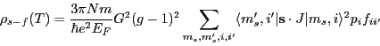
where ![]() is the exchange constant,
is the exchange constant, ![]() is the Bose factor
is the Bose factor
![]() and
and ![]() is the
Fermi function
is the
Fermi function
![]() . The program rhoso1ion can be used to calculate this
resistivity for magnetic ions in a crystal field. The wavefunctions
. The program rhoso1ion can be used to calculate this
resistivity for magnetic ions in a crystal field. The wavefunctions ![]() are taken from the file levels.cef output by so1ion. The matrix elements of
are taken from the file levels.cef output by so1ion. The matrix elements of
![]() are calculated according to
the formulae of Dekker [30]. rhoso1ion calculates only the sum in the above equation, however.
The constant coefficient
are calculated according to
the formulae of Dekker [30]. rhoso1ion calculates only the sum in the above equation, however.
The constant coefficient
![]() is set to unity, or may be specified using
the option -rho0 or -r. The syntax is otherwise the same as cpso1ion. For example, to
calculate the resistivity from 10 to 100 K in 1 K steps with
is set to unity, or may be specified using
the option -rho0 or -r. The syntax is otherwise the same as cpso1ion. For example, to
calculate the resistivity from 10 to 100 K in 1 K steps with ![]()
![]() .cm, the command rhoso1ion 10 100 1 -r 0.2 can be used. Alternatively, for comparison with data, rhoso1ion 1 2 rhoexp.dat
-r 0.2 can be used. Note that as the temperature dependence of the resistivity in this case is mainly a
function of the Bose and Fermi functions, at high temperatures where all
.cm, the command rhoso1ion 10 100 1 -r 0.2 can be used. Alternatively, for comparison with data, rhoso1ion 1 2 rhoexp.dat
-r 0.2 can be used. Note that as the temperature dependence of the resistivity in this case is mainly a
function of the Bose and Fermi functions, at high temperatures where all ![]() crystal field levels are
thermally occupied, the resistivity will saturate to a value
crystal field levels are
thermally occupied, the resistivity will saturate to a value ![]() .
.
Exercises:
![\includegraphics[angle=0,width=1.0\textwidth]{figsrc/10KCEFspectrum.eps}](img106.png)